Splits tab

This tab is used to define all the parameters affecting the samples : the matrices, the classes, the pairing, the number of splits, etc.

This step exists in the pipeline mainly because of the nature of metabolomic data, or more generally biological data : it has few samples, but hundreds or thousands of features per sample. This situation is called fat data, as opposed to big data where there is tens of thousands of samples to learn from and each of them is of a reasonable size. See more below in the Splits section.

• Files
• Define Classification designs
• Samples pairing
• Balancing
  • Balancing in automate script
• Splits
  • Limitation
• Generate the splits file

Files

For data and metadata, the supported files are excel or csv. If the error “Rows must have an equal number of columns” occurs when loading a file, it means that some lines don’t have cells for all columns.

Normalization for Progenesis

Use this to specify if you are using a matrix produced by Progenesis or another matrix with samples as lines and features as columns. Also, if it is from Progenesis, it can be either the raw abundance values or the normalized.

Not Progenesis

Use this to specify the use of a data matrix not produced by Progenesis. The required format for those matrices is samples as lines and features as columns. The related metadata file needs to have a column corresponding to the samples names present in the data matrix. This column serves as a connector between the samples data and their corresponding metadata.

Retention time below 1min

Progenesis produced matrices identify their features with the retention time and the m/z ratio. It allows a filtering on features detected before 1 minute of acquisition (most likely noise, artefacts, other non-biologically relevent element). It prevents potential bias.

Data

Data matrix input

Metadata

Metadata matrix input, is optional but necessary for pairing, and often offers clearer classes.

The user is responsible for the format of the input files (if not progenesis) and matrices. The optimal choices are :

• csv format
• each line of the metadata should correspond to a line of the data, and vice versa. Meaning there should only be informations on the exact same samples in both files. (It does not have to be in the same order.) It is not mandatory, but providing different matrices/files than that can result in malfunctioning. The tool is built to try to cover as many variations of experiment as possible, but we might have missed some. If you did not provide that formatting and encounter problems you can modify your files and try again.

It is considered the data file will only contain the samples which are to be used for an experiment. We are starting to support the presence in the metadata file of extra samples not included in an experiment.

Your samples name identifiers must be string (text), there is not yet a safeguard in case of numbers.

Define Classification designs

The PICO only allows binary classification, so the classification designs add more flexibility. In ML litterature, the three following terms are often used as synonyms. In the context of ML applied to biological data, we needed them to reflect three slightly different things. There might have been some mixing up during development in the names of variables and function. Always refer to this section to clarify.

Classes

Classes are categories of sample groups in the data. A typical example is the column that contains a diagnosis.

Labels

Designate a group of class(es).

Targets

Targets are the values the models will output as prediction. They correspond to labels.

Pratical example

An experiment with data from two different studies (studyA, studyB) and three diagnosis (High Symptoms, Low Symptoms and Controls). The metadata contains two columns of interest : Studies and Diagnosis, both of them selected as ‘target columns’ (meaning they will be used to define what targets will be predicted by the models). Potential classes are : studyA, studyB, High Symptoms, Low Symptoms and Controls, or a combination of those.

Classification design 1 (StudyAHigh_vs_StudyALow)

• classes : studyA__High Symptoms and studyA__Low Symptoms
• labels :
  • StudyAHigh for studyA__High Symptoms
  • StudyALow for studyA__Low Symptoms
• targets :
  • 0 for StudyAHigh
  • 1 for StudyALow

Classification design 2 (1Symptoms_vs_0AllControls) In this example, we consider that studyA__High Symptoms has peculiarities due to the design of the study and thus should not be included.

• classes : studyA__Low Symptoms, studyB__High Symptoms, studyB__Low Symptoms, studyA__Controls and studyB__Controls
• labels (the ‘0’ and ‘1’ added at the beginning are optionnal, they are used to decide which label gets target 0 vs 1):
  • 1Symptoms for (studyA__Low Symptoms & studyB__High Symptoms & studyB__Low Symptoms)
  • 0AllControls for (studyA__Controls & studyB__Controls)
• targets :
  • 0 for label 0AllControls
  • 1 for label 1Symptoms

Those are only two example but there could be many. Moreover, a user simply wanting to compare diagnosis could select only the column “Diagnosis” as ‘target column’ and have High Symptoms, Low Symptoms and Controls as potential classes.

By default, if the user provides a Progenesis file as data, the PICO will parse the file and select the second header of the table as classes. (The first header being Raw abundance and Normalized abundance, and the third header being the name of the samples.) Otherwise, the PICO will read the metadata file and displays the columns names. If there are not the column names expected, please retry uploading the metadata in the section A. The user can then choose which (one or multiple) column(s) to use as class(es). In other word, which information the model will try to predict. If the user choose multiple columns, the classes will be a combination of the values of those columns. The user will also need to select which column of the metadata file contains the unique ID or sample names. It is used by the PICO to link the metadata information to each unique sample in the data.

After this step, starts the creation of classification designs. With each target column the user chose, the section updates and displays the possibilities (original classes are separated from each other by ‘__’). The user has to name the new group of classes by defining a label.

If there is a checkbox without a value in the list of possible class, it means certain lines of the metadata matrix have empty cells for the selected target columns. Do not select it (the checkbox witout value), it will cause problems.

Once it is filled, clicking on the ‘Add’ button will add this new design to the setup of the experiment and clear the fields. The user can then repeat the process to define a new design. The ‘Reset’ button in the block of defined classification designs will erase all designs already defined.

All the designs will be run with the same:

• Number of splits
• Percentage of samples in the test set
• Pairing group
• Algorithms

Samples pairing

This section allows the user to select a column in the metadata that will be used to fine-tune the division of train and test set. Sample pairing is meant to deal with a situation common in clinical studies: crossover design. In these studies, the experimental design will include multiple sampling of each participant, each sampling corresponding to a different treatment. In those cases, we must ensure that all samples belonging to one individual are either used to train or to test the model. This prevents biasing the algorithm towards learning the specificities of each participant instead of what distinguishes the labels. The pairing section aims to group samples that are identified as a cluster by a selected column in the metadata.

Balancing

Rebalancing the classes can be made for each classification design.

Balancing in automate script

Computing balancing value for a design (classA_vs_classB).

classA must be the one with the highest number of samples.

• find total number of examples for the design : nbr_A + nbr_B = Tot
• for classA, round to ceil(nbr_A/Tot*100) to obtain it ratio = ratioA (60)
• for classB, round to floor(nbr_B/Tot*100) to obtain it ratio = ratioB (40)
• substract 50 from ratioA, it gives you the interval of difference
• Then divide this interval in 5 (parameter arbitrarly defined and hardcoded in the tool)
  • this should produce a list of numbers, which are now the options of value to rebalance (ex: 0, 2, 4, 6, 8)
• to see the impact of each value option on the ratio, take each option, substract from the higher ratio and add to the lowest
  • 60:40 (starting point), 58:42, 56:44, 54:46 and 52:48 (closest to 50:50)
• If you wish to rebalance to 54:46, you will need to indicate the value “6” to the function metabo_controller.set_balance_correction_for_experiment()

Splits

To apply machine learning to fat data, the strategy used here is to produce multiple splits. It is not a widespread practice in common machine learning applications, some confusion might arise when talking about it to machine learners. (It might be confused with cross-validations folds or boostrap aggregating.) The splitting process we are implementing here is the production of multiple train-test dataset division completely independent of each other.

The train-test repartition of 20% of samples in test set and 80% in train set is quite common for metabolomic datasets. Often machine learning experiments will use a ratio closer to 30%-70%, but it always depends on the number of samples needed to train the model.

For the number of splits, a more complete run will be startt at 20 to 25 splits. Using 5 splits can be interesting when doing small tests of the parameters because it will be faster. However, it will not cover all the samples in a testing setting. The computing to display the graph is triggered the first time by uploading the data file, it takes by default the value of 25 splits.

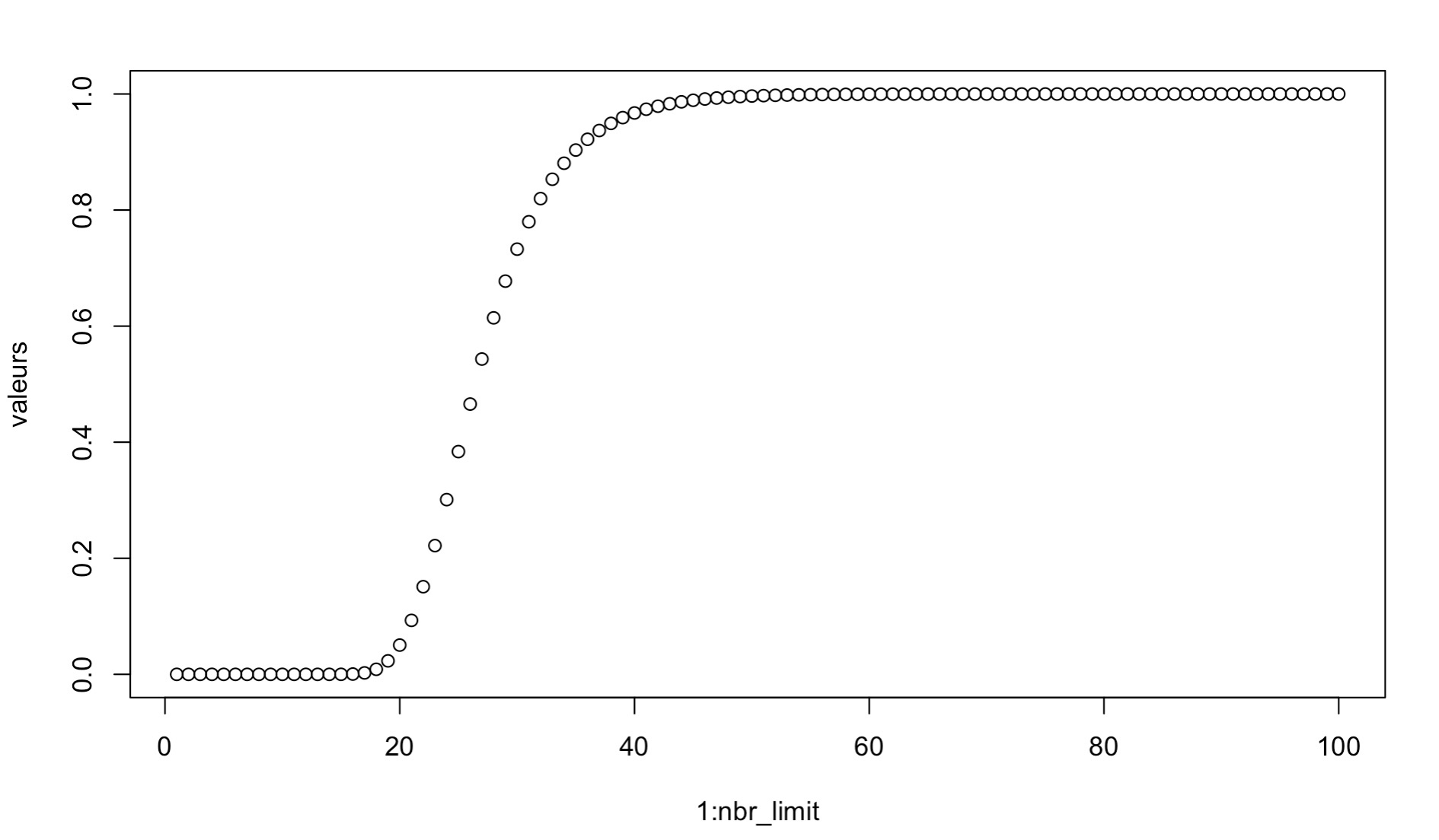
We determined that the appropriate number of splits for an experiment can be found using a Markov chain process. Indeed, the probability that all samples are seen in the test set, i.e. the probability that a sample is never in the test set, follow a Markov chain.

Math example with equations and figure

P(X<1) (values) as a function of the number of splits n (1:nbr_limit) with m=250 samples and a test proportion of 0.2 (k=50)

Limitation

The computing of “a” and “b” values for splits choice number is only made on the full data matrix (i.e. total number of samples provided in the file). It makes those values conservative estimates for classification designs including less samples. Indeed, the higher the number of samples, the higher the number of splits needs to be to see most of them. If a classification design involves less samples, the “a” and “b” values are the minimum and the real (not computed) values are higher.

Generate the splits file

Once all the parameters, the samples id and target columns, and at least one classification design are set, you can run the splits’ computation by clicking on the CREATE button. All the parameters will be saved and for each split, the unique identification of the samples belonging in the train or test set will be saved. No data or metadata is saved, the matrices for the machine learing are retrieved with the samples unique identification when needed.